Z Tests | Z Tests and t Tests | Biostatistics Study Notes

The Z-test compares the sample statistic to the population specified by the null hypothesis and measures how many standard errors the difference is. Since standardized statistics follow or approximate a standard normal distribution under H₀, critical values and p-values can be determined.

Distinguishing an Individual Z Score from a Z Statistic for a Mean#

An individual Z score indicates how many population standard deviations X is away from the population mean. In testing the mean, we treat X̄ and use its standard deviation, the standard error σ/√n, as the denominator.

individual z-score

Z=\frac{X-\mu}{\sigma}

Standardization of sample mean

Z=\frac{\bar X-\mu}{\sigma/\sqrt n}

Symbol	Meaning
X	individual observations
X̄	sample mean of n observations
μ	population mean
μ₀	The population mean specified by H₀
σ	known population standard deviation
n	sample size
σ/√n	standard error of the sample mean

Why the Z Test Is Valid#

If the population is normally distributed, the sample mean is also normally distributed. Even if it is non-normal, it can be approximated by the central limit theorem with appropriate conditions and sufficient n.

Expected value of sample mean

E(\bar X)=\mu

variance of sample mean

\operatorname{Var}(\bar X)=\frac{\sigma^2}{n}

standard error

\operatorname{SE}(\bar X)=\frac{\sigma}{\sqrt n}

Z statistic under H₀

Z=\frac{\bar X-\mu_0}{\sigma/\sqrt n}\sim N(0,1)

Z-test conditions#

The sampling distribution of the statistic is normal or can be reasonably approximated by a normal distribution.
Random sampling and independence of observations. Paired or clustered data require methods appropriate to that dependence structure
In the Z test of the mean, the population standard deviation σ is known. When σ is unknown and replaced by s, use a t test as a general rule.
Even with a large sample, unknown σ does not become known.

Hypotheses and Decision for a One-Sample Mean#

two-sided

H_0:\mu=\mu_0,\qquad H_1:\mu\ne\mu_0

right-tailed

H_0:\mu\leq\mu_0,\qquad H_1:\mu>\mu_0

left-tailed

H_0:\mu\geq\mu_0,\qquad H_1:\mu<\mu_0

Direction	Rejection condition	p-value
two-sided	\|Zobs\| ≥ z₁₋α⁄₂	2P(Z≥\|Zobs\|)
right-tailed	Zobs ≥ z₁₋α	P(Z≥Zobs)
left-tailed	Zobs ≤ zα	P(Z≤Zobs)

Z-test for independent two-sample means#

For two independent groups, we treat the mean difference X̄₁−X̄₂. If the population variance is known, due to independence, the variance of the mean difference is the sum of the variances of the two groups.

variance of mean difference

\operatorname{Var}(\bar X_1-\bar X_2)=\frac{\sigma_1^2}{n_1}+\frac{\sigma_2^2}{n_2}

Independent two-sample Z statistic

Z=\frac{(\bar X_1-\bar X_2)-\Delta_0}{\sqrt{\sigma_1^2/n_1+\sigma_2^2/n_2}}

For a test of no difference, Δ₀=0. Since covariance cannot be ignored in matched data, we analyze the differences between each pair.

Confidence Interval: Solve the Same Standardized Equation for μ#

A two-tailed (1−α) confidence interval is obtained by solving for the unknown μ from the median area 1−α of a standard normal distribution.

median probability

P\!\left(-z_{1-\alpha/2}\leq\frac{\bar X-\mu}{\sigma/\sqrt n}\leq z_{1-\alpha/2}\right)=1-\alpha

Solve μ

P\!\left(\bar X-z_{1-\alpha/2}\frac{\sigma}{\sqrt n}\leq\mu\leq\bar X+z_{1-\alpha/2}\frac{\sigma}{\sqrt n}\right)=1-\alpha

confidence interval

\bar X\pm z_{1-\alpha/2}\frac{\sigma}{\sqrt n}

In the 95% interval, z₀.₉₇₅=1.96. The confidence level is the long-term proportion of intervals containing the true μ when the same procedure is repeated, not the probability that μ falls within the completed fixed interval.

Overlapping the H₀ and H₁ Distributions#

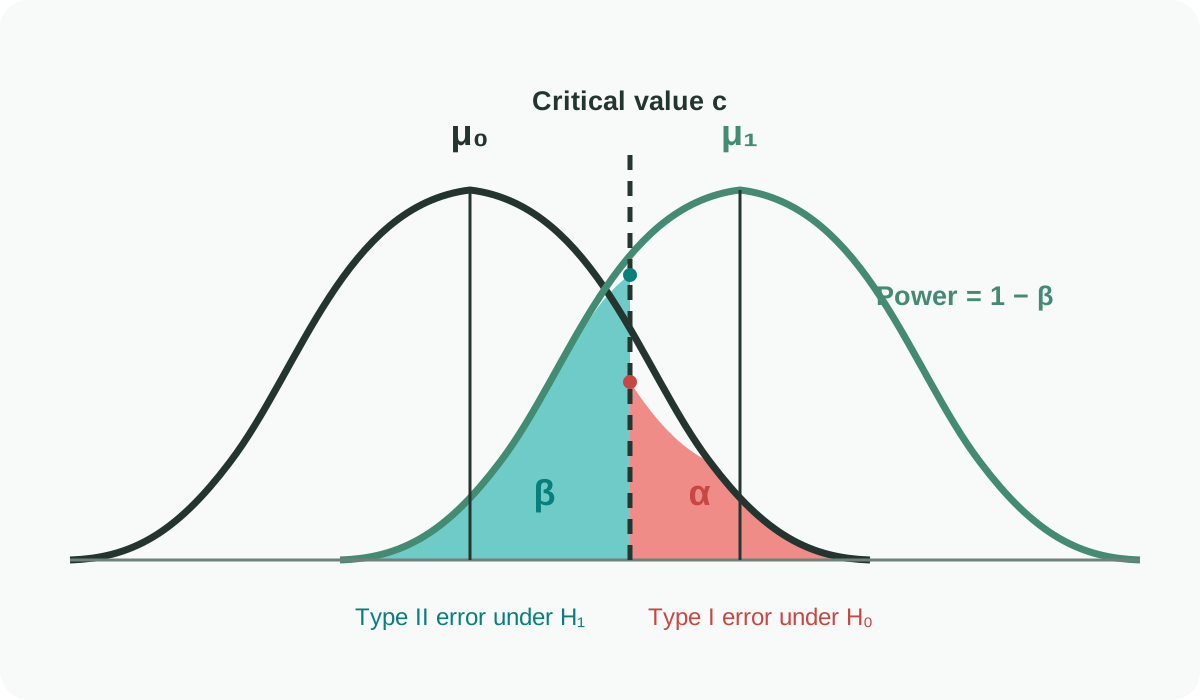
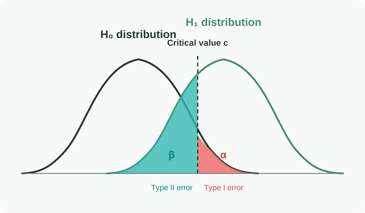
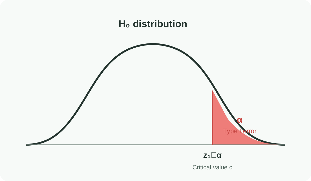
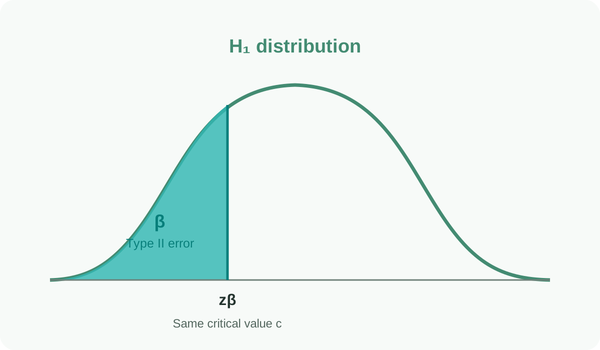
α is the area that exceeds the critical point and is falsely rejected when H₀ is true, and β is the area that cannot cross the same critical point when a certain H₁ (μ=μ₁) is true.

Overlapping sampling distributions under H₀ and H₁; the area to the right of the common critical value is Type I error α under H₀, while the area to its left is Type II error β under H₁ — α and β use the same critical boundary but are calculated under the H₀ distribution and a specified H₁ distribution, respectively.Source: Recreated for this site from the original notes

Determine the Right-Tailed Critical Point from α under H₀#

Right tail of the H₀ sampling distribution, with the area beyond the critical value representing Type I error α — For a right-tailed test, choose the critical value under H₀ so that the area to its right equals α.Source: Recreated for this site from the original notes

Z value of critical point

z_{1-\alpha}=\frac{c-\mu_0}{\sigma/\sqrt n}

critical sample mean

c=\mu_0+z_{1-\alpha}\frac{\sigma}{\sqrt n}

β for a Right-Tailed Test: View the Same Critical Point under H₁#

H₁ sampling distribution with the area to the left of the same critical value representing Type II error β — Place the same critical value on the H₁ distribution; the area to its left, where H₀ is not rejected, is β.Source: Recreated for this site from the original notes

Standardized critical point under H₁

z_\beta=\frac{c-\mu_1}{\sigma/\sqrt n}

Type 2 error

\beta=P_{\mu_1}(\bar X\leq c)=\Phi(z_\beta)

statistical power

1-\beta=1-\Phi(z_\beta)=\Phi(-z_\beta)

Sample Size: Control α While Maintaining Power#

By subtracting two equations that use the same critical point c for H₀ and H₁, c disappears and the required sample size can be found.

Eliminate critical points

z_{1-\alpha}-z_\beta=\frac{\mu_1-\mu_0}{\sigma/\sqrt n}

Symmetry of normal distribution

z_\beta=-z_{1-\beta}

1 sample side sample size

n=\left[\frac{(z_{1-\alpha}+z_{1-\beta})\sigma}{\mu_1-\mu_0}\right]^2

Round up n. This formula is for a one-sample, one-tailed, mean Z test with known σ, with z₁₋α⁄₂ for two-sided.

Supplementary example: sample size and detectable difference

In a study comparing hip ultrasound alpha angle between preterm and term infants, we planned a sample size for each group to detect a mean difference of 3° or 2°, with σ = 4.9°, two-sided α = 0.05, and a power of 80%.

Standard error of the mean difference between two independent groups

\operatorname{SE}(\bar X_1-\bar X_2)=\sigma\sqrt{\frac{2}{n}}

Sample size for each group

n=2\left[\frac{(z_{1-\alpha/2}+z_{1-\beta})\sigma}{\delta}\right]^2

Detectable difference δ	Effect size d=δ/σ	Normal approximation	Published study
3°	Approximately 0.61	Approximately 42 hips in each group	43 hips
2°	Approximately 0.41	Approximately 95 hips in each group	96 hips

Reference: Hockett C, et al. J Pediatr Orthop. 2024;44(1):e25–e29. doi:10.1097/BPO.0000000000002540.

How the Formula Determines Sample Size#

change	necessary n	reason
α↓	increase	Type 1 errors are suppressed and boundaries become stricter.
β↓（power↑）	increase	We need information so we don't miss the real difference.
σ↑	increase	loud noise
\|μ₁−μ₀\|↑	decrease	Big differences are easy to spot

Deriving Power from the Same Framework#

One-sided statistical power

1-\beta=\Phi\!\left(\frac{\sqrt n\,|\mu_1-\mu_0|}{\sigma}-z_{1-\alpha}\right)

two-sided approximation

1-\beta\approx\Phi\!\left(\frac{\sqrt n\,|\mu_1-\mu_0|}{\sigma}-z_{1-\alpha/2}\right)

For strict two-sided power, we add the probability that the H₁ distribution falls into both the left and right rejection regions. An increase in n or effect increases the power, and an increase in σ or a decrease in α decreases the power if other conditions are held constant.

Overlapping H₀ and H₁ distributions showing Type I error α, Type II error β, and statistical power 1−β — With other conditions fixed, moving the critical value changes α and β in opposite directions; reducing overlap between the distributions increases power.Source: Recreated for this site from the original notes