Chi-Square Distribution | Probability Distributions

The chi-square distribution (χ² distribution) describes a random variable that is the sum of the squares of multiple independent standard normal variables. Because it converts the standardized deviation in each direction into a non-negative total variation, it is closely related to variance estimation, the chi-square test, and the F distribution, which will be treated later.

How is the chi-square distribution created?#

If Z₁, Z₂, ..., Zν are ν standard normal variables that are mutually independent, then U, which is the sum of the squares of each one, follows a chi-square distribution with ν degrees of freedom. Each additional square of an independent standard normal variable increases the degree of freedom by one.

Each variable follows a standard normal distribution

Z_i\sim N(0,1),\qquad i=1,2,\ldots,\nu

The sum of squares creates a chi-square distribution

U=\sum_{i=1}^{\nu}Z_i^2\sim\chi^2_{\nu}

symbol	meaning
Zᵢ	i standard normal variable
U	Sum of squares of all standard normal variables
ν	Degree of freedom. number of independent squared terms
χ²ν	Chi-square distribution with ν degrees of freedom

Why is the chi-square value never less than 0?#

Since each Zᵢ is not negative when squared, the sum of squares U must also be greater than or equal to 0. With one degree of freedom, the chi-square variable is the square of one standard normal variable. Intuitively, it can be thought that the values on the left and right sides of the normal curve are mapped to the positive range by squaring, but the shape of the density also changes due to variable transformation.

Understanding the shape of one degree of freedom from the standard normal curve#

With ν=1 degrees of freedom, U=Z², and Z follows the standard normal distribution. After squaring both negative and positive values of the standard normal curve, they are mapped to 0 or higher; for example, Z=−2 and Z=2 both become U=4. Therefore, it is thought that the probabilities on both the left and right sides are moved to the positive half axis and combined.

However, since squaring changes not only the sign but also the interval between values, density cannot be found by directly adding the left and right heights. Variable conversion requires a correction factor, and this is the "correction term" mentioned in the original note.

square a standard normal variable

U=Z^2,\qquad Z\sim N(0,1)

Chi-square density with 1 degree of freedom

f_U(u)=\frac{\phi(\sqrt{u})+\phi(-\sqrt{u})}{2\sqrt{u}}=\frac{1}{\sqrt{2\pi u}}e^{-u/2},\qquad u>0

symbol	meaning
φ(z)	Probability density at position z of standard normal distribution
√u、−√u	Two original Z values that, when squared, give u
1/(2√u)	Correction factor for density by square transformation

How do degrees of freedom change the shape of the distribution?#

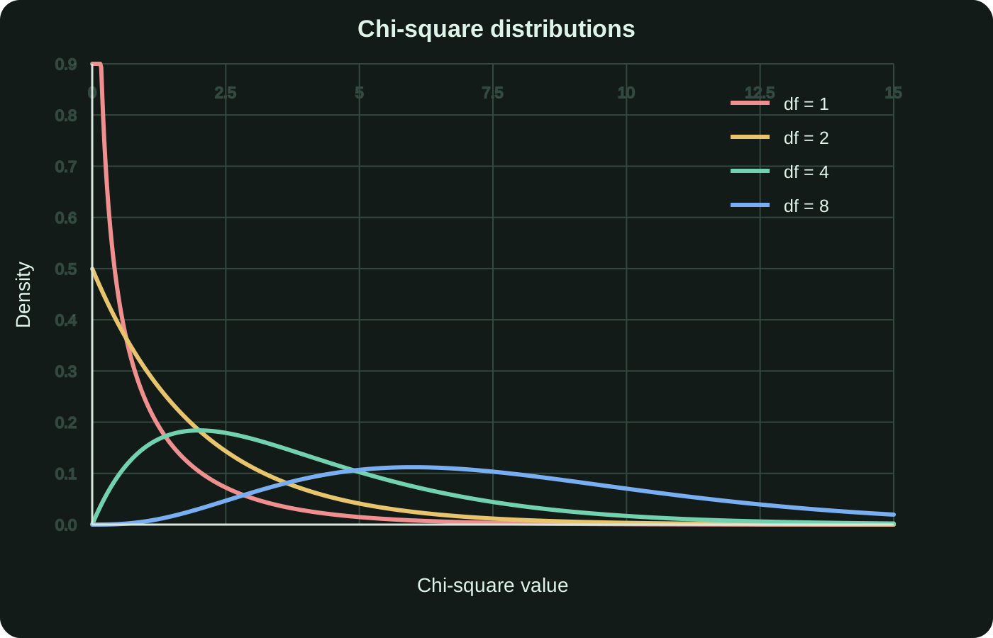
When the degrees of freedom are low, the chi-square distribution is strongly skewed to the right, with many values clustered around 0 and a long tail on the right. As the degrees of freedom increase, the number of independent square terms increases, the center moves to the right, and the relative distortion decreases, approaching a bell shape, but the value never goes below 0.

Why does it become more bell-shaped as the degrees of freedom increase?#

A chi-square variable with ν degrees of freedom is the sum of ν mutually independent Zᵢ². Each Zᵢ² can be thought of as a chi-square variable with one degree of freedom, so increasing the degrees of freedom is equivalent to adding more independent squared terms with the same distribution. This is the same idea as the "sum of many independent random variables" that the central limit theorem deals with.

More precisely, each Zᵢ² has a mean of 1 and a variance of 2, so the sum U has a mean of ν and a variance of 2ν. As ν increases, the distribution obtained by subtracting the mean ν from U and dividing by the standard deviation √(2ν) approaches the standard normal distribution. Therefore, the unstandardized chi-square curve widens as it moves to the right, becoming less skewed and more bell-shaped.

\frac{U-\nu}{\sqrt{2\nu}}\xrightarrow{d}N(0,1)\qquad(\nu\to\infty)

Chi-square density curves with 1, 2, 4, and 8 degrees of freedom; the center moves right and relative skewness decreases as the degrees of freedom increase — The chi-square distribution is strongly right-skewed at low degrees of freedom. As the degrees of freedom increase, its center moves right and its shape becomes more symmetric.Source: Created for this site from the chi-square density function

nature	χ² distribution with ν degrees of freedom
possible values	0 to positive infinity
average	ν
dispersion	2ν
shape	It is distorted to the right in low degrees of freedom, and becomes relatively symmetrical as degrees of freedom increase.

Chi-square distribution and sample variance#

When n independent observations are drawn from a normal population, the adjusted ratio of the sample variance S² to the population variance σ² follows a chi-square distribution with n−1 degrees of freedom. This is an important basis for estimating population variance from sample variance.

Standardize using known population mean

\sum_{i=1}^{n}\left(\frac{X_i-\mu}{\sigma}\right)^2\sim\chi_n^2

When using the sample mean

\frac{(n-1)S^2}{\sigma^2}=\sum_{i=1}^{n}\left(\frac{X_i-\bar X}{\sigma}\right)^2\sim\chi_{n-1}^2

symbol	meaning
Xᵢ	i-th observation
μ、σ²	Normal population mean and variance
X̄、S²	sample mean and sample variance
n	sample size
n−1	degrees of freedom remaining after using the sample mean

Probability density function of chi-square distribution#

The probability density function of a chi-square distribution with ν degrees of freedom is: This formula determines the height and shape of the curve for each degree of freedom, and the total area under the curve is 1.

f(u)=\frac{1}{2^{\nu/2}\Gamma(\nu/2)}u^{\nu/2-1}e^{-u/2},\qquad u>0

symbol	meaning
f(u)	Probability density of chi-square distribution at location u
u	Possible values of chi-square variable greater than 0
ν	Chi-square distribution degrees of freedom
Γ	Gamma function that makes the total area under the density curve 1
e	The base of the natural logarithm of approximately 2.71828

Supplement: Derivation of chi-square density function

Step 1: Derive 1 degree of freedom

Let Z be a variable with standard normal distribution and define U=Z². For any u>0, z²=u has two solutions: z=√u and z=−√u. Since two Z values map to the same U value, density conversion adds both contributions.

standard normal density

\phi(z)=\frac{1}{\sqrt{2\pi}}e^{-z^2/2}

Inverse function and its derivative

z_1=\sqrt{u},\quad z_2=-\sqrt{u},\qquad \left|\frac{dz_j}{du}\right|=\frac{1}{2\sqrt{u}}

add two densities

f_U(u)=\phi(\sqrt{u})\frac{1}{2\sqrt{u}}+\phi(-\sqrt{u})\frac{1}{2\sqrt{u}}

After reduction

f_U(u)=\frac{1}{\sqrt{2\pi u}}e^{-u/2},\qquad u>0

|dz/du| is the Jacobian correction of variable transformation. It is not sufficient to directly add the heights on the left and right sides of the normal curve, as this reflects the expansion and contraction of the interval between values by the square. The result is the chi-square density with one degree of freedom.

Another way to check: Compare the chi-square density with 1 degree of freedom and the standard normal density

You can also check the reverse from two known densities. Standardize the general normal distribution to μ=0, σ=1, and set the degree of freedom ν of the chi-square density to 1.

General normal density

f_X(x)=\frac{1}{\sigma\sqrt{2\pi}}\exp\!\left[-\frac12\left(\frac{x-\mu}{\sigma}\right)^2\right]

Assign μ=0, σ=1

\phi(x)=\frac{1}{\sqrt{2\pi}}e^{-x^2/2}

General chi-square density

f_{\chi^2_\nu}(u)=\frac{1}{2^{\nu/2}\Gamma(\nu/2)}u^{\nu/2-1}e^{-u/2}

Use ν=1 and Γ(1/2)=√π

f_{\chi^2_1}(u)=\frac{1}{\sqrt{2\pi}}e^{-u/2}u^{-1/2}

If we put u=x², the exponential part e^(−u/2) of the chi-square density corresponds to e^(−x²/2) of the standard normal density, and the extra u^(−1/2) is the scale correction due to the square transformation. This is a complete correspondence to the explanation that "a correction term remains even after replacing χ² with x²".

Second step: Expand to ν independent square terms

Let U=Z₁²+⋯+Zν². Since repeating density convolution is cumbersome, we use a moment-generating function (MGF). The MGF of the sum of independent random variables is the product of their respective MGFs.

MGF of the square of one standard normal variable

M_{Z^2}(s)=E\!\left(e^{sZ^2}\right)=(1-2s)^{-1/2},\qquad s<\frac12

sum of ν independent square terms

M_U(s)=\prod_{i=1}^{\nu}M_{Z_i^2}(s)=(1-2s)^{-\nu/2}

The corresponding chi-square density

f_U(u)=\frac{1}{2^{\nu/2}\Gamma(\nu/2)}u^{\nu/2-1}e^{-u/2},\qquad u>0

The final MGF matches a Gamma distribution with shape parameter ν/2 and scale parameter 2, resulting in a chi-square density function with ν degrees of freedom.

symbol	Meaning in derivation
φ(z)	standard normal density function
\|dz/du\|	Jacobian absolute value correcting density with variable transformation
Mᵤ(s)	moment generating function of U
E	Expected value calculation
Π	Multiply the MGF of each independent squared term
Γ	Gamma function