
CHAPTER 02 · TOPIC 09
Poisson Distribution
Model event counts in a fixed interval and connect the rate parameter to binomial limits and exponential waiting times.
On this page
- In what cases should you use it?
- What does the parameter λ represent?
- probability mass function
- How does λ change the shape of the distribution?
- mean and variance are equal
- Commonly Used Probabilities
- Approximation by binomial distribution
- Relationship with exponential distribution
- Independent Poisson Counts Are Additive
A Poisson distribution is a discrete probability distribution that describes the number of times an event occurs within a given time, area, volume, or other interval.
In what cases should you use it?#
- Count the number of times X occurs within a fixed interval
- Events occur with a roughly constant average rate of occurrence
- The number of occurrences of non-overlapping intervals can be considered independent.
- You can ignore the probability that it will happen more than once in a very short interval.
What does the parameter λ represent?#
λ is the expected number of occurrences within the selected observation interval. If the average incidence per unit interval is r and the length of the observation interval is t, then λ=rt, and if you change the length of the interval, λ will also change.
| symbol | meaning |
| X | Number of occurrences within the selected interval |
| x | Possible values of X |
| λ | Expected number of occurrences within the selected interval |
| r | Average incidence per unit interval |
| t | Observation interval length |
probability mass function#
Since X takes only non-negative integers, a probability mass function is used instead of a continuous probability density function. The following formula is the probability that an event will occur exactly x times within the interval.
| part of the expression | meaning |
| P(X=x) | Probability of occurrence exactly x times within a fixed interval |
| e^(−λ) | Probability that it will never occur within the interval |
| λ^x | The part about x events and the average number of occurrences |
| x! | a factorial term that adjusts the order of events x times |
How does λ change the shape of the distribution?#
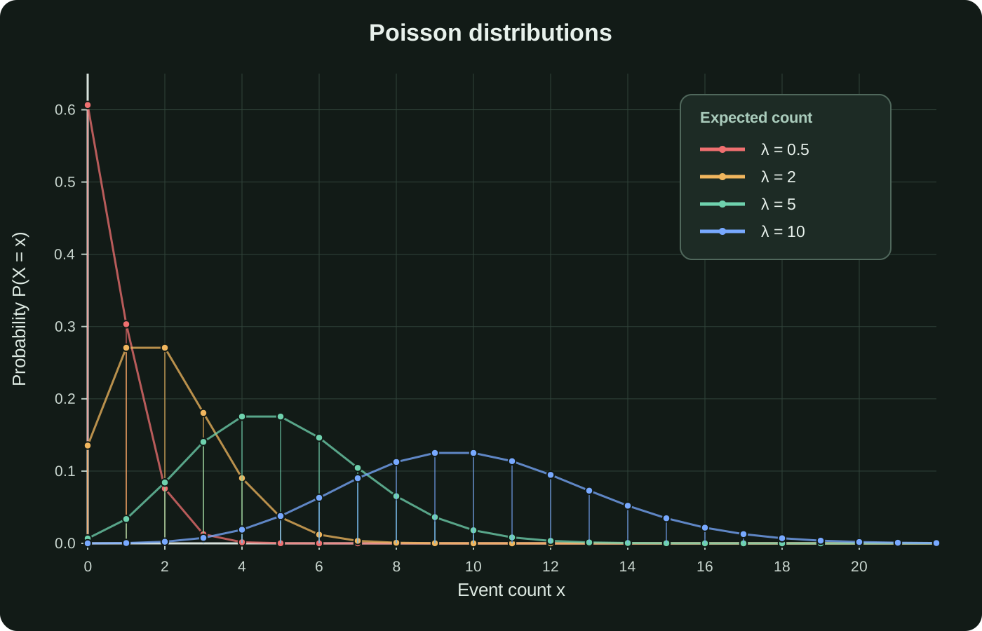
When λ is small, the probability is concentrated to 0 and a small number of times and skewed to the right. As λ increases, the center shifts to the right, increasing the range and reducing relative distortion. The points in the diagram are the actual integer values of X, and the lines are just to help distinguish points from the same distribution.
mean and variance are equal#
In the Poisson distribution, both the expected value and the variance are λ. As λ increases, not only the number of averages but also the absolute variation increases, and the standard deviation becomes √λ.
Commonly Used Probabilities#
The probability that an event will never occur is particularly important, as it immediately determines the probability that it will occur at least once from co-events.
Supplement: Deriving Poisson's formula from the binomial distribution
Step 1: Divide the observation interval into many small intervals
Assume that events occur an average of λ times in the entire interval, and divide it into n short intervals. When n is large, the probability of occurrence of each interval is approximately λ/n, and the probability of occurrence more than once can be ignored, so it can be temporarily treated as a binomial trial.
Step 2: Separate the Expression into Parts with Evaluatable Limits
Stage 3: Find three limits
Increase n while keeping x fixed. The sorting ratio approaches 1, the index limit approaches e^(−λ), and the fixed index correction approaches 1.
Approximation by binomial distribution#
If n is large and p is small in the binomial distribution, and λ=np is a moderate size, the number of successes can be approximated by Poisson(λ). Suitable for events that occur only on a small number of occasions.
Relationship with exponential distribution#
In a Poisson process with occurrence rate r, the number of occurrences N(t) within length t follows Poisson(rt), and the waiting time T until the next event follows Exp(r). One measures the number of times, the other measures the interval.
Independent Poisson Counts Are Additive#
If the counts of different sources are independent, the total count also follows a Poisson distribution, and the population is the sum of the counts of each source. Naturally integrate counts from different time periods, regions, and sources.