Exponential Distribution | Probability Distributions

The exponential distribution is a continuous probability distribution that describes waiting times between independent events occurring at a constant average rate.

In what cases should you use it?#

It is used to measure the time until the next call or customer arrives, or the failure time of equipment assuming a certain failure rate. Check that your data is not only latency, but also that the average incidence is roughly constant and that events in different time intervals can be considered independent.

Definition of exponential distribution#

If the random variable X is the waiting time until the next event and the average occurrence rate is λ, then X follows an exponential distribution with a parameter λ.

Distribution notation

X\sim\operatorname{Exp}(\lambda),\qquad \lambda>0

probability density function

f(x)=\begin{cases}\lambda e^{-\lambda x},&x\ge 0,\\0,&x<0.\end{cases}

symbol	meaning
X	Wait time until next event
x	Possible values of X
λ	Average incidence rate per unit time
f(x)	Probability density of waiting time around x
e	base of natural logarithm

How does λ change the curve?#

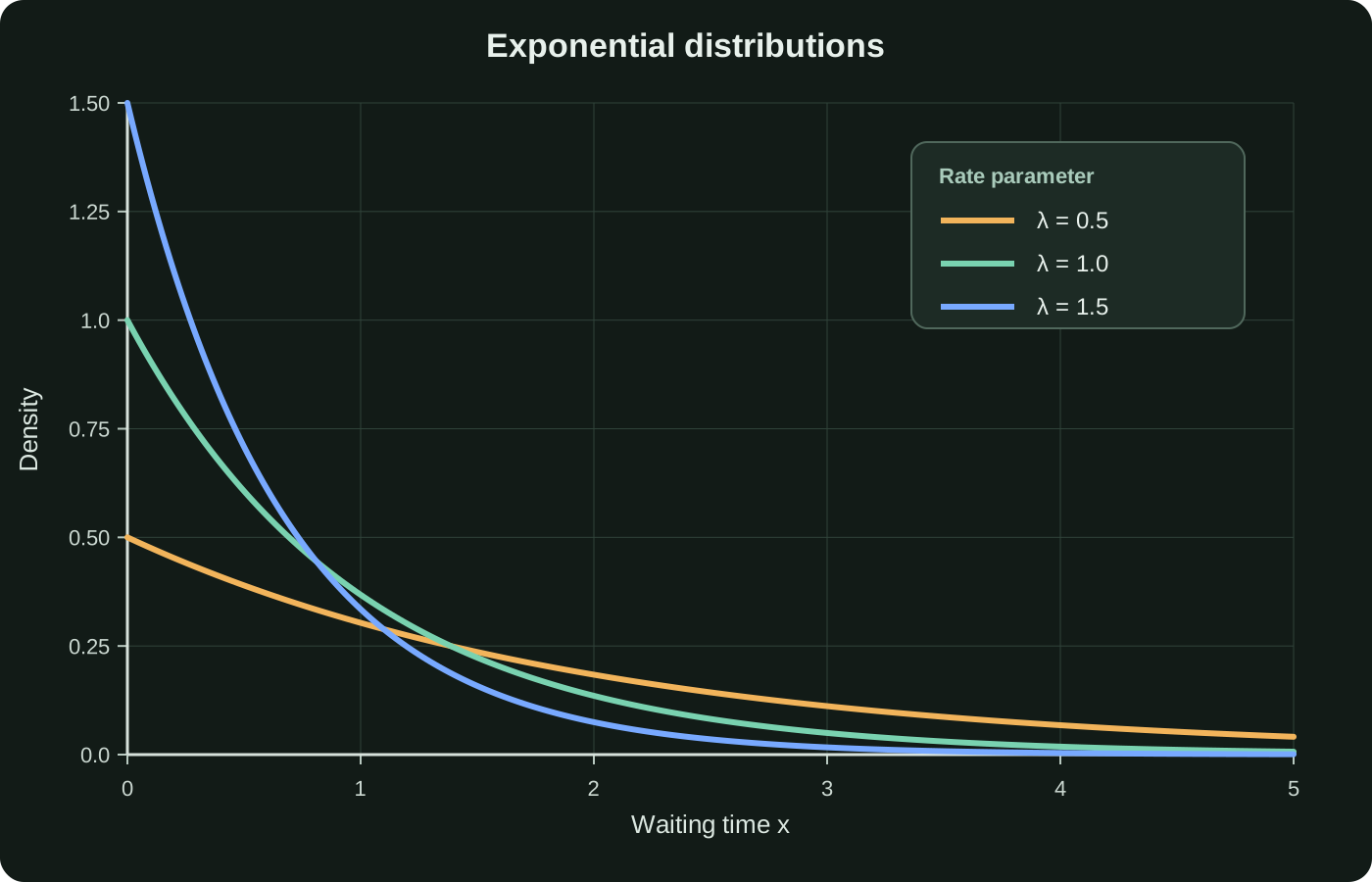
The density is f(0)=λ at x=0 and then decreases with latency. The larger λ, the more frequent the event, the faster the curve drops from a higher point, and the shorter the typical waiting time.

Exponential density curves with rates 0.5, 1.0, and 1.5; a larger rate gives a higher starting point and a faster decline — A larger rate means events occur more frequently on average, so waiting times concentrate closer to 0. The total area under each curve is 1.Source: Created for this site from the exponential density function

Find probability from density#

Since it is a continuous distribution, the probability of a single point is 0. The probability that an event will occur within a certain amount of time, or the probability that it will not occur even after that period of time, is calculated using the area under the curve.

Cumulative Distribution Function

F(x)=P(X\le x)=1-e^{-\lambda x},\qquad x\ge0

survival function

S(x)=P(X>x)=e^{-\lambda x},\qquad x\ge0

Probability of falling in the interval

P(a<X\le b)=F(b)-F(a)=e^{-\lambda a}-e^{-\lambda b}

symbol	meaning
f(x)	probability density at position x
F(x)	Cumulative probability that waiting time is less than or equal to x
S(x)	Probability that the event will not occur even if x is exceeded
a、b	Endpoints of the interval where 0≤a<b

Average waiting time and variation#

Occurrence rate and average waiting time are inverses of each other. The larger λ, the smaller the average and variation of the waiting time.

Expected value

E(X)=\frac{1}{\lambda}

variance and standard deviation

\operatorname{Var}(X)=\frac{1}{\lambda^2},\qquad \operatorname{SD}(X)=\frac{1}{\lambda}

Memoryless#

Exponential distributions are memoryless. Given that no event has occurred after waiting s hours, the probability of waiting for more than t is the same as the probability of waiting more than t from the beginning.

P(X>s+t\mid X>s)=P(X>t)=e^{-\lambda t}

Supplement: Deriving exponential distribution from short time intervals

Divide a time of length x into n short intervals Δt=x/n. For a constant occurrence rate λ, the probability that an event does not occur in each interval is approximately 1−λx/n.

No events in each section

P(\text{no event in }\Delta t)\approx 1-\lambda\frac{x}{n}

No event in all n intervals

P(X>x)\approx\left(1-\lambda\frac{x}{n}\right)^n

Make the interval as small as possible

S(x)=P(X>x)=\lim_{n\to\infty}\left(1-\lambda\frac{x}{n}\right)^n=e^{-\lambda x}

This limit first gives the survival function. Subtracting it from 1 gives you the cumulative distribution function, and differentiating it with x gives you the probability density function.

From survival function to cumulative probability

F(x)=1-S(x)=1-e^{-\lambda x}

From cumulative probability to density

f(x)=F'(x)=-S'(x)=\lambda e^{-\lambda x}

Supplement: Why the average waiting time is 1/λ

The expected value of a non-negative random variable can be expressed as the area under the survival function. Integrating S(x)=e^(−λx) yields 1/λ.

E(X)=\int_0^{\infty}S(x)\,dx=\int_0^{\infty}e^{-\lambda x}\,dx=\frac{1}{\lambda}

Relationship with Poisson process#

If the number of occurrences N(t) in time t follows a Poisson distribution with mean λt, then the time until the first event X follows an exponential distribution with parameter λ. Waiting more than t is the same as not having the event occur at all within time t.

Number of occurrences

N(t)\sim\operatorname{Poisson}(\lambda t)

waiting time

P(X>t)=P(N(t)=0)=e^{-\lambda t}

Relationship with survival time analysis#

In survival time analysis, the exponential distribution is a model with a constant λ hazard rate. The hazard rate represents the instantaneous probability that an event will occur in a short period of time, given that you have survived until time x.

h(x)=\frac{f(x)}{S(x)}=\lambda