F Distribution | Probability Distributions

The F-distribution comes from the first letter of R. A. Fisher's last name. A distribution that is obtained by dividing two mutually independent chi-square variables by their degrees of freedom and taking the ratio of the two, and is mainly used to compare the relative magnitudes of two independent amounts of variation.

How is the F distribution created?#

Let U and V be mutually independent chi-square variables, and let the degrees of freedom be ν1 and ν2, respectively. If we divide U and V by each degree of freedom and then take the ratio, F follows an F distribution with ν₁ degrees of freedom in the numerator and ν₂ degrees of freedom in the denominator.

two independent chi-square variables

U\sim\chi^2_{\nu_1},\qquad V\sim\chi^2_{\nu_2},\qquad U\perp V

Create F distribution

F=\frac{U/\nu_1}{V/\nu_2}\sim F_{\nu_1,\nu_2}

symbol	meaning
U、V	Two mutually independent chi-square variables
ν₁	Numerator degrees of freedom corresponding to U
ν₂	Denominator degrees of freedom corresponding to V
U/ν₁、V/ν₂	Average variation of each chi-square variable divided by degrees of freedom
Fν₁,ν₂	F distribution with two degrees of freedom, numerator and denominator
⊥	represents that two random variables are independent

Why doesn't the F value become less than 0?#

Both U and V are sums of squares, so they are not negative. F, which calculates the ratio by dividing by the positive degrees of freedom, also takes only positive values. F=1 indicates that the average fluctuations in the numerator and denominator are equal, F>1 indicates that the numerator is large, and F<1 indicates that the denominator is large.

F\sim F_{\nu_1,\nu_2}\quad\Longrightarrow\quad \frac{1}{F}\sim F_{\nu_2,\nu_1}

How do the two degrees of freedom affect the shape?#

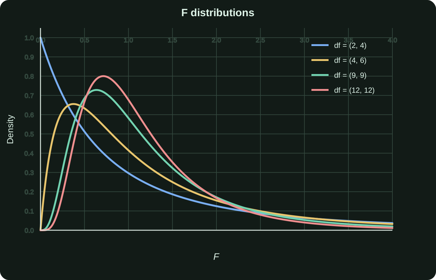
The F distribution is typically right-skewed and has a long tail on the right. The specific shape is determined by both the numerator degree of freedom ν₁ and the denominator degree of freedom ν₂. If the degrees of freedom are low, the variance estimation will be unstable, and the distribution will be wide and the right tail will be thick. As the number of degrees of freedom increases, the ratio generally clusters around 1.

F density curves with numerator and denominator degrees of freedom 2 and 4, 4 and 6, 9 and 9, and 12 and 12 — The F distribution is usually right-skewed. As both degrees of freedom increase, the curve becomes more concentrated near F=1. The legend lists numerator and denominator degrees of freedom in that order.Source: Created for this site from the F density function

Probability density function of F distribution#

The F distribution with numerator degrees of freedom ν₁ and denominator degrees of freedom ν₂ has the following probability density function. Since two degrees of freedom appear simultaneously in the coefficient, index, and denominator, changing just one will change the shape of the curve.

f(x)=\frac{\Gamma\!\left((\nu_1+\nu_2)/2\right)}{\Gamma(\nu_1/2)\Gamma(\nu_2/2)}\left(\frac{\nu_1}{\nu_2}\right)^{\nu_1/2}x^{\nu_1/2-1}\left(1+\frac{\nu_1}{\nu_2}x\right)^{-(\nu_1+\nu_2)/2},\quad x>0

symbol	meaning
f(x)	Probability density of F distribution at position x
x	Possible values of F random variable greater than 0
ν₁、ν₂	Numerator and denominator degrees of freedom
Γ	Gamma function used for normalization coefficient of density function

Supplement: Derivation of F density function

Step 1: Start with two independent chi-square variables

Let U~χ²ν₁, V~χ²ν₂, and let U and V be independent. Define X=(U/ν₁)/(V/ν₂) and leave the auxiliary variable Y=V.

Variable conversion

X=\frac{U/\nu_1}{V/\nu_2},\qquad Y=V

Inverse transformation

U=\frac{\nu_1}{\nu_2}XY,\qquad V=Y

Jacobian

\left|\frac{\partial(u,v)}{\partial(x,y)}\right|=\frac{\nu_1}{\nu_2}y

Since U and V are independent, the joint density is the product of the two chi-square densities. Substituting the inverse transformation and multiplying by the Jacobian gives the joint density of X and Y.

f_{X,Y}(x,y)=f_U\!\left(\frac{\nu_1}{\nu_2}xy\right)f_V(y)\frac{\nu_1}{\nu_2}y

Step 2: Integrate and eliminate the auxiliary variable Y

Integrating for all y>0 gives the marginal density of X. If we rearrange the part related to y, the integral becomes a Gamma integral again.

f_X(x)=\int_0^{\infty}f_{X,Y}(x,y)\,dy

\int_0^{\infty}y^{(\nu_1+\nu_2)/2-1}\exp\!\left[-\frac{y}{2}\left(1+\frac{\nu_1}{\nu_2}x\right)\right]dy

By simplifying with the Gamma integral formula and rearranging the constants, we can obtain the F density function described in the main text. The F density is not a separately assumed formula, but is derived from two independent chi-square densities, ratio definitions, and variable transformations.

symbol	Meaning in derivation
X	F random variable being derived
Y	Auxiliary variable equal to V
fX,Y	Simultaneous density of X and Y
∂(u,v)/∂(x,y)	Jacobian determinant of variable transformation

Relationship between F distribution and t distribution#

If T follows a t distribution with ν degrees of freedom, then T² follows an F distribution with 1 numerator degree of freedom and ν denominator degrees of freedom. This is because when the numerator Z of T is squared, it becomes a chi-square distribution with 1 degree of freedom, and the denominator originally contains U/ν.

Starting from the definition of t

T=\frac{Z}{\sqrt{U/\nu}},\qquad Z^2\sim\chi_1^2

When squared, it becomes F distribution.

T^2=\frac{Z^2/1}{U/\nu}\sim F_{1,\nu}

Why do the two-sided probabilities come together?#

The t distribution is symmetrical around 0. If the total significance level of a two-tailed test is α, then the left and right tails are each α/2. When squared, both T≤−|t| and T≥|t| are reflected in T²≥t², so the left and right probabilities are combined into one right tail of the F distribution. This is the exact meaning of the statement "the probability doubles because both sides overlap".

Events on both sides merge after squaring

P(|T|\ge t)=P(T\le -t)+P(T\ge t)=P(T^2\ge t^2)

Two-tailed t-test and two-tailed F-test

P(|T_\nu|\ge t_{\nu,1-\alpha/2})=\alpha=P(F_{1,\nu}\ge t_{\nu,1-\alpha/2}^{\,2})

Critical value relationship

F_{1,\nu;1-\alpha}=t_{\nu;1-\alpha/2}^{\,2}

Supplement: From the density function, it is derived that T² follows the F distribution

Step 1: Set the Numerator Degrees of Freedom to 1

In the density function of the F distribution, set the numerator degree of freedom ν₁=1, the denominator degree of freedom ν₂=ν, and organize the coefficients using Γ(1/2)=√π and (1/ν)^(1/2)=1/√ν.

General density of F distribution

f_{F_{\nu_1,\nu_2}}(y)=\frac{\Gamma((\nu_1+\nu_2)/2)}{\Gamma(\nu_1/2)\Gamma(\nu_2/2)}\left(\frac{\nu_1}{\nu_2}\right)^{\nu_1/2}y^{\nu_1/2-1}\left(1+\frac{\nu_1}{\nu_2}y\right)^{-(\nu_1+\nu_2)/2}

Substitute ν₁=1, ν₂=ν

f_{F_{1,\nu}}(y)=\frac{\Gamma((\nu+1)/2)}{\Gamma(1/2)\Gamma(\nu/2)}\left(\frac{1}{\nu}\right)^{1/2}y^{-1/2}\left(1+\frac{y}{\nu}\right)^{-(\nu+1)/2}

Simplify with Γ(1/2)=√π

f_{F_{1,\nu}}(y)=\frac{\Gamma((\nu+1)/2)}{\sqrt{\pi\nu}\,\Gamma(\nu/2)}y^{-1/2}\left(1+\frac{y}{\nu}\right)^{-(\nu+1)/2},\quad y>0

Step 2: Compare with the density of the t-distribution

If we replace t² with y in the t density with ν degrees of freedom, everything except y^(-1/2) matches the density of F(1, ν). This additional factor is not an arbitrary constant, but a Jacobian that corrects for changes in the horizontal axis scale due to the square transformation.

f_{T_\nu}(t)=\frac{\Gamma\!\left((\nu+1)/2\right)}{\sqrt{\pi\nu}\,\Gamma(\nu/2)}\left(1+\frac{t^2}{\nu}\right)^{-(\nu+1)/2}

Step 3: Squaring Maps Two t Values to the Same F Value

If Y=T², each y>0 has two elements, t=√y and t=−√y. For the density of Y, it is necessary to collect the probabilities on both the left and right sides of the t distribution, and the absolute value of the derivative of the inverse transformation t=±√y is 1/(2√y).

Square transformation and two inverse functions

Y=T^2,\qquad t_1=\sqrt{y},\quad t_2=-\sqrt{y}

Horizontal scale correction

\left|\frac{dt_1}{dy}\right|=\left|\frac{dt_2}{dy}\right|=\frac{1}{2\sqrt{y}}

density after squared

f_Y(y)=\frac{f_T(\sqrt{y})+f_T(-\sqrt{y})}{2\sqrt{y}}

Since the t distribution is symmetrical, f_T(−√y)=f_T(√y). 2 added on both sides and 2 in the derivative cancel each other out, leaving 1/√y=y^(−1/2).

Utilizing the symmetry of the t-distribution

f_Y(y)=\frac{2f_T(\sqrt{y})}{2\sqrt{y}}=f_T(\sqrt{y})y^{-1/2}

Substitute t density

f_Y(y)=\frac{\Gamma\!\left((\nu+1)/2\right)}{\sqrt{\pi\nu}\,\Gamma(\nu/2)}y^{-1/2}\left(1+\frac{y}{\nu}\right)^{-(\nu+1)/2}=f_{F_{1,\nu}}(y)

Derivation result

T\sim t_\nu\quad\Longrightarrow\quad T^2\sim F_{1,\nu}

symbol	Meaning in derivation
T	t random variable with ν degrees of freedom
Y=T²	Non-negative random variable after square transformation
fT	Probability density function of t distribution
fY	Probability density function of Y after squared
1/(2√y)	Jacobian correction by differentiating t=±√y with y
F(1,ν)	F distribution with numerator degree of freedom 1 and denominator degree of freedom ν

Can F be considered an extension of t?#

If the numerator degree of freedom is 1, the F statistic is the square of the t statistic, and the F test can be thought of as a two-tailed t-test rewritten as a right-sided test that only looks at positive values. The general F distribution allows the numerator degree of freedom to be greater than 1, allowing multiple effects to be tested simultaneously. In this sense, it is an extension of the squared t-test to multiple degrees of freedom, but it cannot be said that all F distributions are the same as one t distribution.

Comparison method	question to answer	Information obtained
Overall F test	Are there at least one difference in the means of the groups?	Determine overall differences, but do not directly indicate which groups differ
2 group t test	Are the means of the two specified groups different?	Show the direction of the difference and the details of the pair
Post hoc pairwise comparison	After the overall F is significant, which groups are different?	Multiple sets are compared, but it is necessary to correct for the increase in type 1 error due to multiple comparisons.

With multiple groups, you can first use the F-test to check whether there is an overall difference, and then use pairwise t-type comparisons or post-hoc comparisons to check which groups differ. However, do not repeat too many uncorrected t-tests, and usually use Tukey, Bonferroni, Holm, etc. to control the overall error rate.

Where is the F distribution used?#

Compare two population variances
Compare between-group and within-group variation with ANOVA
Test whether the entire regression model has explanatory power
Comparing the fit improvement of adding parameters in a nested model
Create confidence intervals and tests for variance components