Random Variables and Probability Density | Probability Distributions

A probabilistic model describes what outcomes can arise from a random phenomenon and how likely each outcome is to occur. To handle these mathematically, we use random variables to convert the trial results into numerical values.

What is a random variable?#

A random variable is a function that associates each random trial result with a numerical value. Since the result is not determined before the trial, there is also uncertainty as to what value the random variable will ultimately take.

Why do we need random variables?#

Real-world random outcomes may be events, conditions, written descriptions, etc. that cannot be calculated as is. Random variables select features of interest, represent them symbolically, and define rules for mapping each outcome to a numerical value. This transformation allows us to construct probability distributions and calculate means, variances, and other statistics.

Observe phenomena with uncertainty.
Choose the features you are really interested in.
Its characteristics are represented by symbols such as X.
Define rules for mapping each result to a numerical value.
Create a distribution from the obtained values and probabilities and perform calculations.

Coin flip example#

If you toss a coin twice in a row, there are four possible outcomes: heads, heads, tails, tails, and tails. If we define X as the number of heads, they correspond to 2, 1, 1, and 0, respectively.

X\in\{0,1,2\}

symbol	meaning
X	A random variable that represents the number of heads.
0、1、2	Possible values of X. Possible or realized value

Statistics can also be random variables#

Statistics such as the sample mean and t, χ², and F are calculated from the sample data. Since the sample is not determined before sampling and the statistics change depending on the sample drawn, it can be treated as a random variable.

Discrete and continuous random variables#

Random variables are divided into discrete and continuous types, depending on whether they can enumerate each possible value one by one. Due to this difference, the functions that describe probability are also different.

kinds	Features	example	Description method
discrete type	Possible values can be listed	Number of successes, number of cases, number of hospitalizations	Probability Mass Function (PMF)
Continuous type	Can take values of arbitrary granularity within the range	Height, weight, blood pressure, survival time	Probability density function (PDF)

Probability mass function: discrete type#

A probability mass function (PMF) is used for discrete random variables. This directly represents the probability that X takes a particular value x.

probability of taking a certain value

p(x)=P(X=x)

sum of probabilities of all possible values

\sum_x p(x)=1

symbol	meaning
X	discrete random variable
x	one possible value of X
p(x)	Probability that X takes x
P(X=x)	Probability of the event "X is equal to x"
Σ	sum the probabilities over all possible values of X

Probability density function: continuous type#

For continuous random variables, we use a probability density function (PDF). The height of the curve at a point is the probability density, not the probability of that point itself. The probability of an interval is the area under the density curve.

Difference between probability density and probability#

Probability density is a function that describes how concentrated the possible values of a random variable are around each location. The height of the function at a certain position is the density, and the area under the curve obtained by integrating the density over a certain range is the probability for that interval.

Why can the density exceed 1?#

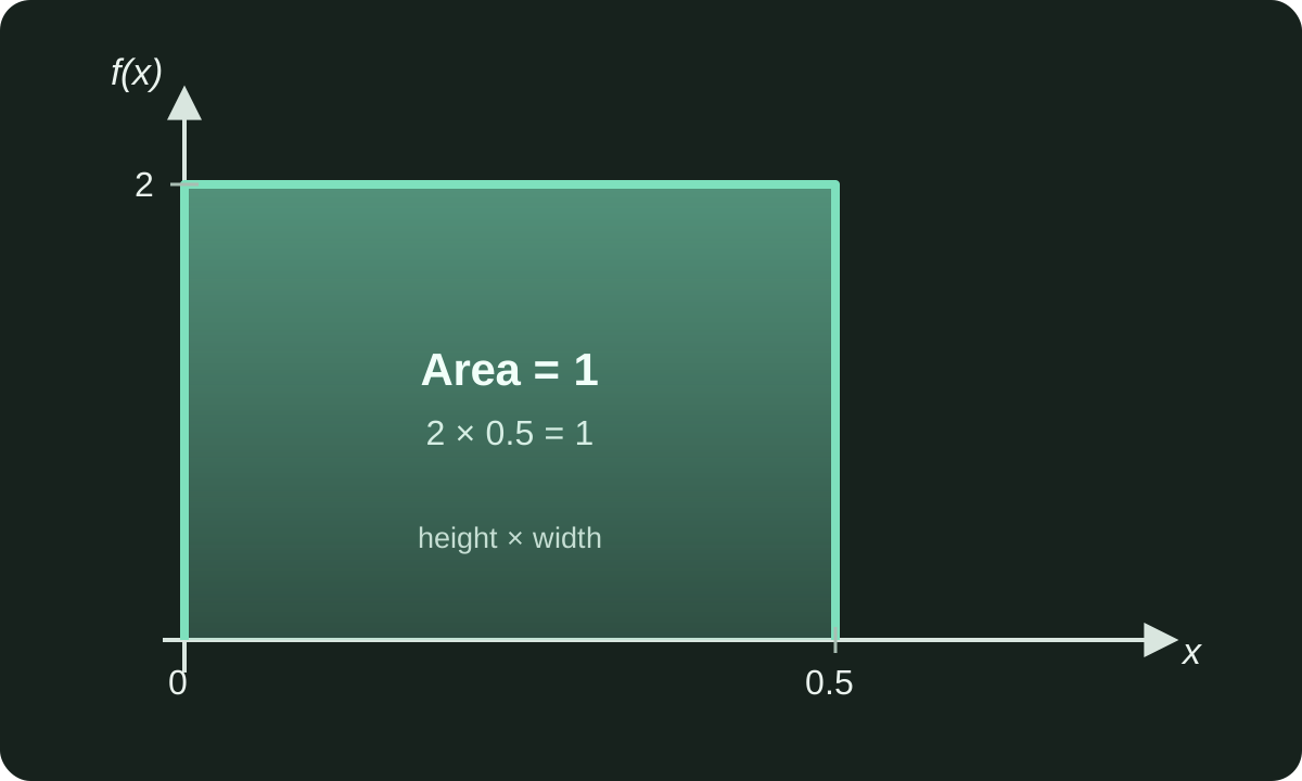
Probability is always between 0 and 1, but probability density can be higher than 1. If the total area under the density curve is 1, then it is a correct probability density function.

For example, suppose X is uniformly distributed between 0 and 0.5. Since the width is only 0.5, the density height can be 2, and the total area is still 0.5 x 2 = 1.

Uniform probability density with height 2 over an interval of width 0.5, giving a total rectangular area of 1 — A density height of 2 does not mean that probability exceeds 1. Probability is the area under the curve, here 2 × 0.5 = 1.Source: Created for this site

density function

f(x)=2,\quad 0\le x\le 0.5

full range probabilities

P(0\le X\le 0.5)=\int_0^{0.5}2\,dx=1

partial probability

P(0\le X\le 0.1)=\int_0^{0.1}2\,dx=0.2

symbol	meaning
f(x)=2	High probability density in this range. Not a probability of 1 point
0.5、0.1	Width of the interval to be calculated
∫	Integrate the density of the specified section as the area under the curve
1、0.2	Interval probability obtained by integration

Probability of 1 point

P(X=x)=0

interval probability

P(a\le X\le b)=\int_a^b f(x)\,dx

Total area under the density curve

\int_{-\infty}^{\infty}f(x)\,dx=1

symbol	meaning
f(x)	Probability density around x. The function value itself is not a probability of one point.
a、b	Lower and upper bounds of the interval for which probability is to be calculated
∫	Area under the density curve in the specified interval
−∞、∞	a range containing all possible values of X

Cumulative Distribution Function#

The cumulative distribution function (CDF) can be used in both discrete and continuous forms and represents the cumulative probability up to x.

common definition

F(x)=P(X\le x)

Continuous representation

F(x)=\int_{-\infty}^{x}f(u)\,du

symbol	meaning
F(x)	Cumulative probability that X is less than or equal to x
f(u)	Probability density function of continuous random variable
u	Variable for integration to avoid confusion with integral upper limit x

Common Probability Distributions#

Types of random variables	Typical distribution
discrete type	binomial, Poisson, hypergeometric
Continuous type	normal distribution, uniform distribution, exponential distribution