t Distribution | Probability Distributions

The t-distribution, also known as the Student's t-distribution, describes the variation in the standardized value of the sample mean when the population standard deviation is unknown. This name comes from William Sealy Gosset, who published under the pseudonym ``Student.''

How is the t-distribution created?#

The t-distribution can consist of a standard normal variable Z and a chi-square variable U that is independent of Z and has ν degrees of freedom. The denominator U/ν represents the uncertainty in estimating the variance from the sample data.

Consists of standard normal variables and chi-square variables

T=\frac{Z}{\sqrt{U/\nu}}\sim t_{\nu}

t-statistic for one-sample mean

T=\frac{\bar X-\mu}{S/\sqrt n}\sim t_{n-1}

symbol	meaning
T	Random variable or t-statistic that follows a t-distribution
Z	standard normal variable
U	chi-square variable independent of Z
ν	degrees of freedom of t distribution
X̄	sample mean
μ	population mean or hypothetical mean
S	Sample standard deviation to estimate unknown σ
n	sample size. For one sample, ν=n−1

Difference between t distribution and standard normal distribution#

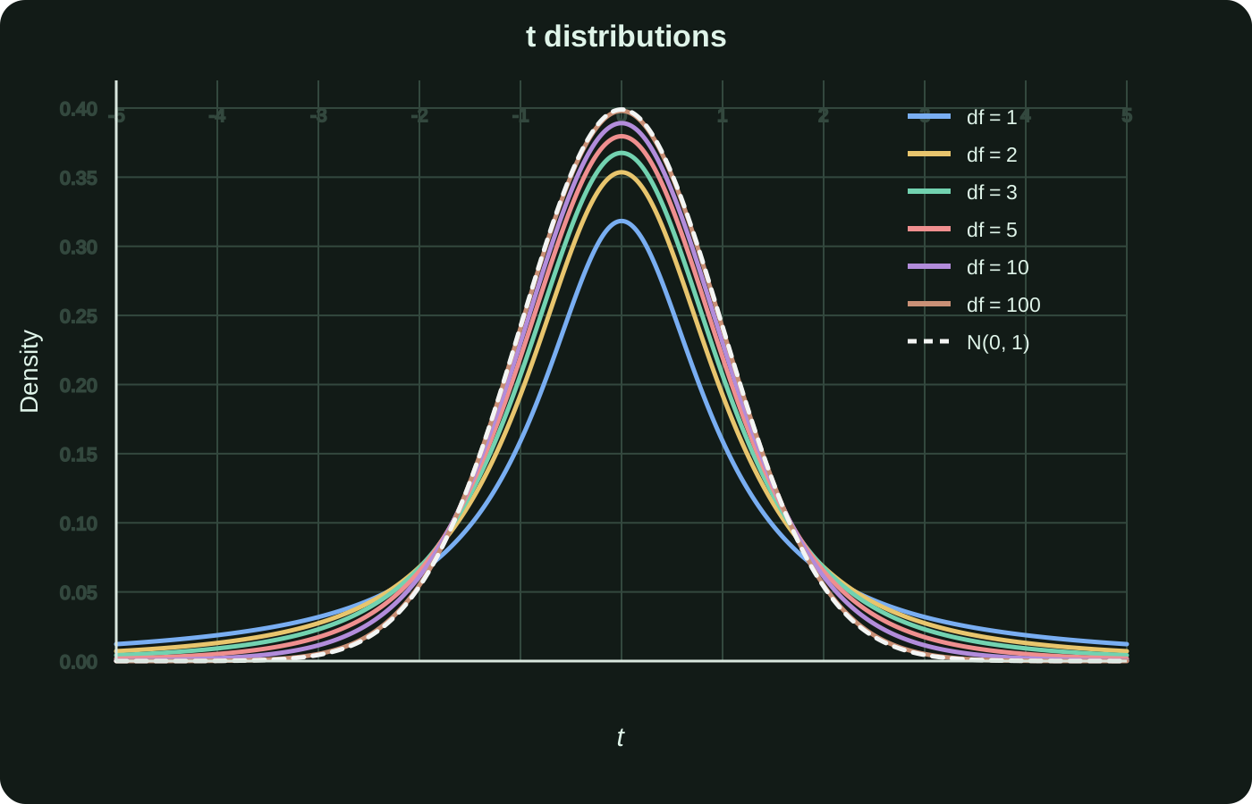
Both the t distribution and the standard normal distribution are symmetrical around 0 and have a bell shape. The difference is that the t-distribution has thicker tails, and values farther from the center are more likely to appear. This reflects the additional uncertainty when the population standard deviation is unknown and is estimated using the sample standard deviation.

comparison	standard normal distribution	t distribution
center	0	0
shape	Left-right symmetrical/bell-shaped	Left-right symmetrical/bell-shaped
hem	relatively thin	The lower the degree of freedom, the thicker it is.
parameter that determines the shape	Fixed to N(0,1)	degree of freedom ν
Main usage scenarios	When the population standard deviation is known or normal approximation is used	When the population standard deviation is unknown and estimated using the sample standard deviation

How do degrees of freedom affect the t-distribution?#

When the degrees of freedom are low, there is less independent information available to estimate the standard deviation, and the uncertainty is greater, so the t-distribution also has thicker tails. As the sample size and degrees of freedom increase, the estimation of the population standard deviation by the sample standard deviation generally becomes more stable, and the t distribution approaches the standard normal distribution.

t density curves with 1, 2, 3, 5, 10, and 100 degrees of freedom compared with the standard normal distribution — At low degrees of freedom, the t distribution has a lower center and heavier tails. As the degrees of freedom increase, it approaches the standard normal distribution N(0,1).Source: Created for this site from the t density function

When should you use the t-distribution?#

Estimate the population mean from one sample mean
Compare the means of two independent groups
Compare mean differences for paired or repeated measures data
Test regression coefficients and correlation coefficients
Create a confidence interval for the population mean or regression coefficient

Probability density function of t distribution#

The t-distribution with ν degrees of freedom has the following probability density function: Since the formula is centered at 0 and includes only t², positive and negative t values with the same absolute value have the same density. This corresponds to the left-right symmetry of the t-distribution.

f(t)=\frac{\Gamma\!\left((\nu+1)/2\right)}{\sqrt{\nu\pi}\,\Gamma\!\left(\nu/2\right)}\left(1+\frac{t^2}{\nu}\right)^{-(\nu+1)/2},\qquad -\infty<t<\infty

symbol	meaning
f(t)	Probability density of t distribution at position t
t	t random variable that takes any real number
ν	degrees of freedom of t distribution
Γ	Gamma function that extends the concept of factorial
π	Pi

Supplement: Derivation of t density function

Step 1: Starting from the definition of the t variable

Assume that Z follows a standard normal distribution and U follows a chi-square distribution with ν degrees of freedom, and both are independent. Define T=Z/√(U/ν) and leave an auxiliary variable V=U to find the density of T.

Variable conversion

T=\frac{Z}{\sqrt{U/\nu}},\qquad V=U

Inverse transformation

Z=T\sqrt{V/\nu},\qquad U=V

Jacobian

\left|\frac{\partial(z,u)}{\partial(t,v)}\right|=\sqrt{\frac{v}{\nu}}

Due to independence, the simultaneous density of Z and U can be expressed as the product of the two densities. Multiplying by Jacobian after variable transformation gives the joint density of T and V.

f_{T,V}(t,v)=f_Z\!\left(t\sqrt{v/\nu}\right)f_U(v)\sqrt{\frac{v}{\nu}}

Step 2: Integrate Out the Auxiliary Variable V

Substituting the standard normal and chi-square densities and integrating for all possible v>0 leaves only T marginal densities.

f_T(t)=\frac{1}{\sqrt{2\pi\nu}\,2^{\nu/2}\Gamma(\nu/2)}\int_0^{\infty}v^{(\nu+1)/2-1}\exp\!\left[-\frac{v}{2}\left(1+\frac{t^2}{\nu}\right)\right]dv

The integral part is in the form of a Gamma integral. It can be simplified directly using the following relation:

\int_0^{\infty}v^{a-1}e^{-bv}\,dv=\frac{\Gamma(a)}{b^a},\qquad a>0,\ b>0

Step 3: Obtain the t Density

f_T(t)=\frac{\Gamma\!\left((\nu+1)/2\right)}{\sqrt{\nu\pi}\,\Gamma\!\left(\nu/2\right)}\left(1+\frac{t^2}{\nu}\right)^{-(\nu+1)/2},\qquad -\infty<t<\infty

Therefore, the t-density is derived from the standard normal density, the chi-square density, and the definition of T. The Gamma function appears because the part that integrates and eliminates the chi-square variable has the form of a Gamma function.

symbol	Meaning in derivation
V	Auxiliary variable left for variable conversion, equal to U
fT,V	Simultaneous density of T and V
∂(z,u)/∂(t,v)	Jacobian determinant of multivariable transformation
a、b	Temporary parameter when applying Gamma integral

Supplement: What is the Gamma function?

The Gamma function extends the concept of factorials to non-positive integers. For a positive integer n, Γ(n)=(n−1)!, so it plays a role similar to a factorial in density functions that include non-integer parameters, such as half the degrees of freedom.

Gamma function definition

\Gamma(a)=\int_0^{\infty}x^{a-1}e^{-x}\,dx,\qquad a>0

recurrence formula

\Gamma(a+1)=a\,\Gamma(a)

Relationship with factorial

\Gamma(n)=(n-1)!,\qquad n=1,2,3,\ldots

Frequently used half-integer values

\Gamma\!\left(\frac12\right)=\sqrt{\pi}

In the density function of the t-distribution, the Gamma function mainly appears in the constant coefficient in the front and adjusts the curve according to the degrees of freedom, making the total area under the density curve 1. You don't need to manually calculate the Gamma function to understand the t-distribution, but knowing its role will help you avoid mistaking Γ for a meaningless decoration.